Comparing 2D population receptive field models on ECoG data from a visual experiment
Author: Malte Lüken (m.luken@esciencecenter.nl)
This examples shows how to fit different population receptive field (pRF) models to electrocorticography (ECoG) data and compare their out-of-sample prediction performance.
A pRF model maps neural activity in a brain region of interest (ROI; e.g., V1 in the human visual cortex) to an experimental stimulus (e.g., a bar moving through the visual field). Here, we use the visual domain as an example, where the pRF is the part of the visual field that stimulates activity in the region of interest. Because the visual field is two-dimensional, the pRF models also have two dimensions.
Because prfmodel uses Keras for model fitting, we need to make sure that a backend is installed before we begin. In this example, we use the TensorFlow backend.
import os
from importlib.util import find_spec
import pandas as pd
# Set keras backend to 'tensorflow' (this is normally the default)
os.environ["KERAS_BACKEND"] = "tensorflow"
# Print parameter DataFrames with three decimals
pd.set_option("display.precision", 3)
if find_spec("tensorflow") is None:
msg = 'Could not find the tensorflow package. Please install it with: pip install "prfmodel[tensorflow]"'
raise ImportError(msg)
Loading the ECoG data
In this example, we use ECoG data recorded from a single subject that is part of the openly available Visual ECoG dataset (Groen et al., 2025). More specifically, we use preprocessed data from a study by Yuasa et al. (2025) that compared the spatial tuning between alpha oscillations (~8-13 Hz) and the broadband response. Here, we only use the broadband response defined as the elevation of the broadband spectrum power (i.e., geometric mean of power in frequency band 70-180 Hz with 1 Hz bins) between stimulus and baseline. We use the full temporal resolution of the experiment (i.e., one sample per bar position, without any further decimation).
We load the dataset and extract the neural response timecourses.
from prfmodel.examples import load_dataset
dataset = load_dataset("visual-ecog-broadband")
response = dataset.response
response.shape
(136, 224)
The dataset has shape (num_channels, num_frames), therefore, the dataset has timecourses for 136 channels and 224 time frames.
Note that the broadband elevation response is expressed as the ratio of the broadband spectrum power between stimulus
and baseline in percentages (i.e., ratio \(\times 100\)), so that a stimulus inside the pRF drives the response upwards.
We can plot the timecourses of all channels all at once.
import matplotlib.pyplot as plt
aspect_ratio = response.shape[1]/response.shape[0]
fig, ax = plt.subplots()
im = ax.imshow(
response,
aspect=aspect_ratio,
cmap="inferno",
vmin=-100,
vmax=1000,
)
ax.set_xlabel("Time frame (in TR)")
ax.set_ylabel("Channel index")
fig.colorbar(im, ax=ax, label="Broadband elevation (in %)");
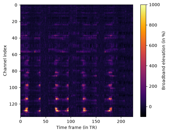
We can already see a regular spiking pattern over time for many channels. The goal of a pRF model is to map these patterns to the experimental stimulus, which we take a look at next.
Loading the stimulus
The experimental stimulus that the responses were measured for is part of the same dataset object.
stimulus = dataset.stimulus
print(stimulus)
PRFStimulus(design=array[224, 100, 100], grid=array[100, 100, 2], frame_duration=0.85, dimension_labels=['y', 'x'])
We can see that the stimulus design has shape (num_frames, num_y, num_x). The number of time frames matches the number
of time frames in the timecourses. The other two dimension contain the energy of the stimulus at each coordinate in the visual field.
The grid contains the visual field coordinates of the design (transformed from screen pixels into degrees of visual angle and resampled to a 100 \(\times\) 100 grid).
We can visualize the stimulus using prfmodel.plotting.animate_2d_prf_stimulus().
from IPython.display import HTML
from prfmodel.plotting import animate_2d_prf_stimulus
ani = animate_2d_prf_stimulus(stimulus, interval=50) # Pause 50 ms between time frames
HTML(ani.to_jshtml())
The stimulus grid spans \(\pm 8.3\) degrees of visual angle in both the x- and y-dimension. The design of this stimulus is different from the typical moving bar stimulus used in pRF experiments (see Fitting a 2D population receptive field model to fMRI data from a visual experiment): It consists of four blocks of 56 time frames each. Every block starts with a full bar sweep along one of the cardinal directions (left to right, top to bottom, right to left, and bottom to top) that takes 28 time frames. This sweep is followed by a diagonal sweep that starts in one of the four corners but is cut short after 12 time frames, just before the bar reaches fixation, and replaced by a blank screen for the remaining 16 time frames of the block. Thus, the subject saw four full cardinal and four truncated diagonal bar sweeps. Because we use the undecimated responses here, the apertures are the binary bar masks of the experiment and no anti-aliasing filter has been applied to them.
Splitting the data for cross-validation
Comparing pRF models on the same data that they were fitted to is misleading because the more complex pRF models that we fit later in this example all add parameters to the Gaussian pRF model. This means that they can overfit, leading to better performance in the in-sample data but worse performance in the out-of-sampel data. To account for overfitting and ensure a fair comparison between pRF models, we perform cross-validation: We fit every model on one half of the timecourses and assess its predictions on the other, held-out half.
The block structure of the stimulus makes a split along the time axis straightforward. Splitting the 224 time frames in the middle gives two halves of two blocks each. The first half holds the left-to-right and top-to-bottom sweeps, the second half the right-to-left and bottom-to-top sweeps. Each half therefore sweeps a full bar both horizontally and vertically across the visual field, so each half constrains the pRF location on its own.
Note: This approach to splitting the data comes with two caveats: First, this is a single split rather than a full cross-validation. Averaging over both directions of the split (fitting on the second half and evaluating on the first) would give a more stable estimate of the out-of-sample fit. Second, the two halves are not independent samples of the same stimulus because the first half sweeps left-to-right and top-to-bottom while the second sweeps right-to-left and bottom-to-top, so any direction-dependent response component (e.g., adaptation along a sweep) decreases out-of-sample performance for every model.
Since PRFStimulus is a frozen dataclass, we can use
dataclasses.replace() to build the two half stimuli from the full one, which keeps the coordinate grid.
from dataclasses import replace
num_channels, num_frames = response.shape
num_split = num_frames // 2
# The first half is used for fitting, the second half is held out for evaluation
response_train = response[:, :num_split]
response_test = response[:, num_split:]
stimulus_train = replace(stimulus, design=stimulus.design[:num_split])
stimulus_test = replace(stimulus, design=stimulus.design[num_split:])
print(stimulus_train)
print(stimulus_test)
PRFStimulus(design=array[112, 100, 100], grid=array[100, 100, 2], frame_duration=0.85, dimension_labels=['y', 'x'])
PRFStimulus(design=array[112, 100, 100], grid=array[100, 100, 2], frame_duration=0.85, dimension_labels=['y', 'x'])
Both halves have 112 time frames for all 136 channels. From here on, we fit every model to response_train with
stimulus_train and report two R-squared values per model: An in-sample score on the first half, and an
out-of-sample score on the held-out second half.
Defining the Gaussian pRF model
Now that we have our response data and stimulus in place, we can create a pRF model to predict a response to this stimulus. We start with the 2D Gaussian pRF model that is based on the seminal paper by Dumoulin and Wandell (2008) with one twist: It assumes that the stimulus (our moving bar) elicits a response that follows a Gaussian shape in two-dimensional visual space. However, ECoG measurements do not follow the shape of the hemodynamic response in the brain (as in fMRI recordings). Therefore, we do not need to convolve the stimulus-encoded pRF response with an impulse response that follows this shape (as in the original model). Finally, a baseline and amplitude parameter shift and scale our predicted response to match the observed ECoG response.
Note that the Gaussian pRF model might not be the best fitting model that captures all phenomena in the observed timecourses. We will fit more complex pRF model variants later in the example and compare them against the Gaussian.
The prfmodel.models.prf.Gaussian2DPRFModel class performs these steps to make a combined prediction. To
exclude the impulse response convolution, se we impulse_model=None.
from prfmodel.models.prf import Gaussian2DPRFModel
# Define pRF model without the impulse response submodel
prf_model = Gaussian2DPRFModel(
impulse_model=None,
)
We define a set of starting parameters to make a combined prediction with our pRF model. We use the full stimulus here to show what the model predicts for the entire experiment.
import numpy as np
import plotly.io as pio
import plotly.express as px
pio.renderers.default = "notebook_connected" # Requires internet connection to work
pio.templates.default = "simple_white"
# Define a set of starting parameters
start_params = pd.DataFrame({
"mu_x": [0.0],
"mu_y": [0.0],
"sigma": [1.0],
"baseline": [0.0],
"amplitude": [1.0],
})
simulated_response = prf_model(stimulus, start_params)
fig = px.line(
pd.DataFrame({
"Time frame (in TR)": np.arange(simulated_response.shape[1]),
"Predicted response": simulated_response[0]
}),
x="Time frame (in TR)",
y="Predicted response",
title="Predicted timecourse",
)
fig.update_layout(height=450)
fig.show()
We can see that for a pRF at the center of the screen (mu_x=0, mu_y=0) with size sigma=1, our model predicts a
response with four larger spikes intertwined with four smaller and sharper spikes. The larger spikes correspond to the cardinal
bar sweeps while the smaller and sharper spikes correspond to the diagonal bar sweeps that stop halfway through.
Note that the predicted response still differs in scale from the broadband elevation response. When fitting the pRF model, we will like need to adjust the model amplitude to adjust for scale differences.
Fitting the Gaussian pRF model
We will fit the pRF model to the first half of our ECoG response data using three stages. We begin with a grid search to find good values for our parameters of interest (mu_x, mu_y, and sigma). Then, we use least squares to estimate the baseline and amplitude of
our model. Finally, we use stochastic gradient descent (SGD) to finetune our model fits using the parameter estiates from the
grid and least squares stage as starting values.
Let’s start with the grid search by defining ranges of mu_x, mu_y, and sigma that we want to construct a grid
of parameter values from. For baseline and amplitude, we only provide a single value so that they will stay constant
across the entire grid.
param_ranges = {
"mu_x": np.linspace(-10, 10, 20), # Range of visual field in experiment
"mu_y": np.linspace(-10, 10, 20),
"sigma": np.linspace(0.005, 20.0, 20),
"baseline": [0.0],
"amplitude": [1.0],
}
For all three parameters, we defined ranges of 20 values that will be used to construct the grid. That is, the grid search will evaluate all possible combinations of these values and return the combination that fits the simulated data best. This will result in a grid containing \(20 ^ 3 = 8000\) parameter combinations. This is still a relatively small grid and we recommend specifying finer grids in practice.
Let’s construct the prfmodel.fitters.GridFitter and perform the grid search. Note that every fitter
is constructed with stimulus_train, so it only ever sees the first half of the experiment. Note also that we set batch_size=20 to let the prfmodel.fitters.GridFitter
evaluate 20 parameter combinations at the same time (which saves us some memory). By default, the loss (i.e., the metric to minimize between model predictions and data) is the negative correlation, which ignores differences in baseline and amplitude between model predictions and observed data. This means the data do not need to be demeaned or converted to percent signal change first, but also that baseline and amplitude cannot be estimated by the grid search itself. We fix them here and estimate them with least squares in the next step.
from prfmodel.fitters import GridFitter
# Create grid fitter object
grid_fitter = GridFitter(
model=prf_model,
stimulus=stimulus_train,
compile_step=True, # Setting 'compile_step=True' speeds up the fitting
)
# Run grid search
_, grid_params = grid_fitter.fit(
data=response_train,
parameter_values=param_ranges,
batch_size=20,
)
We can print the parameters estimated by the grid search.
grid_params
| mu_x | mu_y | sigma | baseline | amplitude | |
|---|---|---|---|---|---|
| 0 | -5.789 | 10.000 | 1.057 | 0.0 | 1.0 |
| 1 | -1.579 | -4.737 | 0.005 | 0.0 | 1.0 |
| 2 | -1.579 | 7.895 | 0.005 | 0.0 | 1.0 |
| 3 | 2.632 | 10.000 | 1.057 | 0.0 | 1.0 |
| 4 | -2.632 | -7.895 | 1.057 | 0.0 | 1.0 |
| ... | ... | ... | ... | ... | ... |
| 131 | -1.579 | -10.000 | 4.214 | 0.0 | 1.0 |
| 132 | -10.000 | -2.632 | 2.110 | 0.0 | 1.0 |
| 133 | -10.000 | -0.526 | 6.319 | 0.0 | 1.0 |
| 134 | -0.526 | -0.526 | 1.057 | 0.0 | 1.0 |
| 135 | 1.579 | 7.895 | 0.005 | 0.0 | 1.0 |
136 rows × 5 columns
We can see that the estimates for mu_x, mu_y, and sigma are one combination in our grid. In the second step,
we also optimize the amplitude of the pRF model together with the baseline using least squares. This adjusts the
scale of our model predictions to scale the observed data.
from prfmodel.fitters import LeastSquaresFitter
# Create least-squares fitter
ls_fitter = LeastSquaresFitter(
model=prf_model,
stimulus=stimulus_train,
)
# Run least squares fit
_, ls_params = ls_fitter.fit(
data=response_train,
parameters=grid_params,
slope_name="amplitude", # Names of parameters to be optimized with least squares
intercept_name="baseline",
)
ls_params
| mu_x | mu_y | sigma | baseline | amplitude | |
|---|---|---|---|---|---|
| 0 | -5.789 | 10.000 | 1.057 | -4.095 | 781.838 |
| 1 | -1.579 | -4.737 | 0.005 | -2.371 | 0.003 |
| 2 | -1.579 | 7.895 | 0.005 | 3.656 | 0.022 |
| 3 | 2.632 | 10.000 | 1.057 | 17.862 | 84.260 |
| 4 | -2.632 | -7.895 | 1.057 | -0.496 | 0.834 |
| ... | ... | ... | ... | ... | ... |
| 131 | -1.579 | -10.000 | 4.214 | 8.213 | 20.312 |
| 132 | -10.000 | -2.632 | 2.110 | 12.944 | 25.260 |
| 133 | -10.000 | -0.526 | 6.319 | 0.232 | 29.929 |
| 134 | -0.526 | -0.526 | 1.057 | -2.251 | 1.677 |
| 135 | 1.579 | 7.895 | 0.005 | 5.591 | 0.051 |
136 rows × 5 columns
We can see that the amplitudes are substantially lower compared to the starting value (and our initial guess) for many channels.
Finally, we use SGD to finetune the parameter estimates. Note that we use an Adapter to optimize the pRF size sigma on the unconstrained log-scale.
from keras import ops
from prfmodel.fitters import SGDFitter
from prfmodel.fitters.adapter import Adapter, ParameterTransform
adapter = Adapter([
ParameterTransform(
parameter_names=["sigma"],
transform_fun=ops.log,
inverse_fun=ops.exp
),
])
sgd_fitter = SGDFitter(
model=prf_model,
stimulus=stimulus_train,
adapter=adapter,
compile_step=True,
)
_, sgd_params = sgd_fitter.fit(data=response_train, init_parameters=ls_params)
sgd_params
| mu_x | mu_y | sigma | baseline | amplitude | |
|---|---|---|---|---|---|
| 0 | -5.180 | 8.758 | 0.600 | -3.988 | 782.764 |
| 1 | -1.577 | -4.738 | 0.005 | -2.371 | 0.004 |
| 2 | -1.576 | 7.895 | 0.005 | 3.656 | 0.022 |
| 3 | 2.653 | 9.998 | 1.055 | 17.883 | 85.240 |
| 4 | -2.422 | -6.869 | 0.365 | -0.536 | 0.384 |
| ... | ... | ... | ... | ... | ... |
| 131 | -1.708 | -10.128 | 4.456 | 8.030 | 21.303 |
| 132 | -10.065 | -2.489 | 2.027 | 13.418 | 26.225 |
| 133 | -9.882 | -0.984 | 6.368 | -0.055 | 29.740 |
| 134 | -0.257 | -0.955 | 1.198 | -2.871 | 1.761 |
| 135 | 1.576 | 7.895 | 0.005 | 5.591 | 0.050 |
136 rows × 5 columns
We can see that some of the SGD parameter estimates for mu_x, mu_y, and sigma have moved away from the grid points.
Now that the core pRF parameters and the auxiliary baseline and amplitude parameters are optimized, we can compare the model predictions against the observed responses. We predict the response to the full stimulus in one call and slice the two halves out of it afterwards. This gives exactly the same result as predicting each half separately, because without an impulse response no model stage carries information between time frames.
pred_response = np.asarray(prf_model(stimulus, sgd_params))
We can quantify how well the predictions align with the observed timecourses using the R-squared metric. This metric indicates the proportion of variance in the observed data explained by our model predictions. We compute it twice: on the first half that the model was fitted to (in-sample) and on the held-out second half (out-of-sample). Since we repeat this for every model variant, we wrap it in a small helper function.
from keras.metrics import R2Score
r2_metric = R2Score(class_aggregation=None) # Don't aggregate score over channels
SPLIT_NAMES = ("In-sample (first half)", "Out-of-sample (second half)")
def score_splits(predicted):
"""Compute in-sample and out-of-sample R-squared for a prediction of the full experiment."""
scores = []
for observed, predicted_half in [
(response_train, predicted[:, :num_split]),
(response_test, predicted[:, num_split:]),
]:
r2_metric.reset_state() # Metric accumulates state across calls
scores.append(np.asarray(r2_metric(observed.T, predicted_half.T))) # Transpose to score across time frames
return dict(zip(SPLIT_NAMES, scores, strict=True))
r_squared = score_splits(pred_response)
We can look at the distribution of R-squared values across channels for both halves.
def r_squared_frame(scores_by_model):
"""Turn a mapping of model name to split scores into a long DataFrame for plotting."""
return pd.concat([
pd.DataFrame({"R-squared": values, "Model": model, "Split": split})
for model, by_split in scores_by_model.items()
for split, values in by_split.items()
])
fig = px.histogram(
r_squared_frame({"Gaussian": r_squared}),
x="R-squared",
facet_col="Split",
nbins=15,
)
fig.for_each_annotation(lambda a: a.update(text=a.text.split("=")[-1])) # Remove 'Split=' from panel titles
fig.update_layout(yaxis_title="Frequency", height=450)
fig.show()
The R-squared values are spread widely across channels in both halves, and the out-of-sample distribution is clearly below the in-sample one. Many channels even have a negative out-of-sample R-squared, meaning the prediction is worse than simply predicting the mean of the held-out half. This can be explained by two things: First, The dataset covers all channels over visual cortex, including ones with little visually driven response. Second, the undecimated timecourses retain the fast fluctuations that the pRF cannot predict and decimation would average out (as Yuasa et al. (2025) did in their paper).
We can plot the predicted and the observed timecourses for the different channels. The shaded area marks the held-out second half, so the left part of each timecourse is the fit and the right part is the prediction.
import plotly.graph_objects as go
y_label = "Broadband elevation (in %)"
colors = pio.templates[pio.templates.default].layout.colorway
time_frames = np.arange(num_frames)
def add_holdout_marker(figure):
"""Shade the held-out second half of the experiment."""
figure.add_vrect(
x0=num_split - 0.5,
x1=num_frames - 0.5,
fillcolor="#000000",
opacity=0.06,
line_width=0,
annotation_text="Held out",
annotation_position="top left",
)
def format_scores(scores_by_model, channel, precision):
"""Format the in- and out-of-sample R-squared of every model for one channel."""
return "<br>".join(
f"{split}: "
+ ", ".join(f"{model} = {by_split[split][channel]:.{precision}f}" for model, by_split in scores_by_model.items())
for split in SPLIT_NAMES
)
def channel_figure(traces, scores_by_model, title, precision=3):
"""Build a per-channel timecourse figure with a slider over channels."""
figure = go.Figure()
# Add the traces for the first channel
for source, (values, style) in traces.items():
figure.add_trace(
go.Scatter(
x=time_frames,
y=values[0],
mode="lines",
name=source,
line={**style, "width": 2},
)
)
# Each slider step replaces the y-values of all traces and updates the title
steps = []
for channel in range(num_channels):
y_values = [values[channel] for values, _ in traces.values()]
scores = format_scores(scores_by_model, channel, precision)
steps.append({
"method": "update",
"label": str(channel),
"args": [{"y": y_values}, {"title.text": f"{title}<br>{scores}"}],
})
add_holdout_marker(figure)
figure.update_xaxes(title_text="Time frame (in TR)")
figure.update_yaxes(title_text=y_label)
figure.update_layout(
sliders=[{"active": 0, "currentvalue": {"prefix": "Channel index: "}, "pad": {"t": 60}, "steps": steps}],
title=f"{title}<br>{format_scores(scores_by_model, 0, precision)}",
margin={"t": 140},
height=600,
)
return figure
fig = channel_figure(
{
"Observed": (response, {"color": "#555555", "dash": "solid"}),
"Gaussian": (pred_response, {"color": colors[0], "dash": "dash"}),
},
{"Gaussian": r_squared},
"Observed and predicted channel response",
)
fig.show()
For many channels, we can see that the observed broadband elevation responses undershoot before and after each spike. This suggests surround suppression and that a model that accounts for a center-surround configuration in the spatial pRF tuning profile is more appropriate to fit these responses.
Defining the DoG pRF model
In their study, Yuasa et al. (2025) use a Difference of Gaussian (DoG; Zuiderbaan et al., 2012) pRF model to fit the broadband elevation response data. The DoG model has two spatial pRF tuning profiles (a center and a surround) that have the same center but different sizes and amplitudes. By subtracting the two profiles, the DoG pRF model can account for surround suppression effects as seen in the response undershoots.
The DoG pRF model is implemented in the DoG2DPRFModel class. The model has parameters
for the shared center of the two Gaussian tuning profiles (mu_x and mu_y), but different sizes and amplitudes for
each profile (sigma_center, sigma_surround and amplitude_center, amplitude_surround).
We first create an instance of the DoG pRF model and set impulse_model=None to skip impulse response convolution.
from prfmodel.models.prf import DoG2DPRFModel
prf_model_dog = DoG2DPRFModel(
impulse_model=None,
)
# We can take a look at the list of model parameters
prf_model_dog.parameter_names
['mu_y',
'mu_x',
'sigma_center',
'sigma_surround',
'amplitude_center',
'amplitude_surround',
'baseline']
We can also make a prediction with the DoG pRF model with some starting parameters to get a feeling for how the suppression effect looks like compared to the Gaussian pRF model.
We can use the helper function init_dog_from_gaussian() to quickly initialize parameters
of the DoG pRF model from the Gaussian pRF model. The function uses the Gaussian parameters as parameters for the center
tuning profile. We only need to specify how much larger the size of the surround
compared to the center profile and how large the amplitude of the surround should be.
from prfmodel.models.prf import init_dog_from_gaussian
# Define a set of starting parameters
start_params_dog = init_dog_from_gaussian(start_params, sigma_ratio=5, amplitude_surround=0.5)
simulated_response_dog = prf_model_dog(stimulus, start_params_dog)
fig = px.line(
pd.DataFrame({
"Time frame (in TR)": np.tile(time_frames, 2),
"Predicted response": np.concatenate([np.asarray(simulated_response[0]), np.asarray(simulated_response_dog[0])]),
"Model": ["Gaussian"] * num_frames + ["DoG"] * num_frames,
}),
x="Time frame (in TR)",
y="Predicted response",
color="Model",
line_dash="Model",
title="Predicted timecourse",
)
fig.update_layout(height=450)
fig.show()
When comparing the predicted responses between DoG and Gaussian pRF model, we can see the undershoots around the spikes in the DoG pRF model.
Fitting the DoG pRF model
Again, we use the parameter estimates from the Gaussian pRF model as starting values for fitting the DoG pRF model.
We only use SGD to fit the DoG pRF model to the first half of the observed broadband elevation response. As starting values we use the parameter estimates from the Gaussian pRF model.
init_params_dog = init_dog_from_gaussian(sgd_params, sigma_ratio=5.0, amplitude_surround=0.5)
Because the default starting values for amplitude_center and amplitude_surround might lead to substantially different
prediction scales for different channels (depending on the other Gaussian pRF parameters), we use least squares to re-adjust
them together with baseline.
ls_fitter_dog = LeastSquaresFitter(
model=prf_model_dog,
stimulus=stimulus_train,
)
_, ls_params_dog = ls_fitter_dog.fit(
response_train,
init_params_dog,
intercept_name="baseline",
slope_name=["amplitude_center", "amplitude_surround"],
)
Now, we use the re-adjusted baseline and amplitude estimates together with the Gaussian parameter estimates as starting values for SGD to finetune all parameters.
adapter_dog = Adapter([
ParameterTransform(
parameter_names=["sigma_center", "sigma_surround"],
transform_fun=ops.log,
inverse_fun=ops.exp
),
])
sgd_fitter_dog = SGDFitter(
model=prf_model_dog,
stimulus=stimulus_train,
adapter=adapter_dog,
compile_step=True,
)
_, sgd_params_dog = sgd_fitter_dog.fit(data=response_train, init_parameters=ls_params_dog)
sgd_params_dog
| mu_x | mu_y | baseline | sigma_center | sigma_surround | amplitude_center | amplitude_surround | |
|---|---|---|---|---|---|---|---|
| 0 | -4.742 | 7.920 | -1.658 | 0.292 | 7.167 | 1053.258 | 4.124 |
| 1 | -1.575 | -4.738 | -2.371 | 0.005 | 0.026 | 0.004 | -0.002 |
| 2 | -1.574 | 7.895 | 3.656 | 0.005 | 0.025 | 0.020 | -0.008 |
| 3 | 2.737 | 10.071 | 18.363 | 1.121 | 3.332 | 88.840 | 2.081 |
| 4 | -2.402 | -6.881 | 2.140 | 0.129 | 4.301 | 0.576 | 2.208 |
| ... | ... | ... | ... | ... | ... | ... | ... |
| 131 | -1.735 | -10.548 | 4.404 | 1.810 | 7.403 | 19.537 | -22.645 |
| 132 | -9.702 | -2.445 | 8.903 | 1.320 | 5.444 | 25.508 | -9.873 |
| 133 | -8.932 | -0.816 | 4.013 | 6.815 | 26.177 | 37.331 | 95.002 |
| 134 | -0.237 | -0.953 | 2.019 | 1.739 | 5.007 | 3.434 | 4.374 |
| 135 | 1.580 | 7.894 | 5.591 | 0.005 | 0.025 | 0.046 | -0.015 |
136 rows × 7 columns
Again, we can compare the responses predicted with the SGD parameter estimates against the observed broadband elevation response, in-sample and out-of-sample.
pred_response_dog = np.asarray(prf_model_dog(stimulus, sgd_params_dog))
r_squared_dog = score_splits(pred_response_dog)
r_squared_models = {"Gaussian": r_squared, "DoG": r_squared_dog}
r_squared_models_df = r_squared_frame(r_squared_models)
fig = px.histogram(
r_squared_models_df,
x="R-squared",
color="Model",
facet_col="Split",
barmode="overlay",
opacity=0.6,
)
# Use the same bins for both models so the histograms are directly comparable
bin_start = np.floor(r_squared_models_df["R-squared"].min() * 20) / 20
fig.update_traces(xbins={"start": bin_start, "end": 1.0, "size": 0.05})
fig.for_each_annotation(lambda a: a.update(text=a.text.split("=")[-1])) # Remove 'Split=' from panel titles
fig.update_layout(yaxis_title="Frequency", height=450)
fig.show()
The DoG pRF model fits the first half better than the Gaussian pRF model. This is not surprising given that it the DoG pRF model has two additional parameters. However, when looking at the out-of-sample predictions, we see that the two models fit the data almost equally well. This suggests that, for many channels, the DoG pRF model was overfitting on the in-sample data and that we cannot reliably fit surround-suppression for those channels (either because it is not present or because it is masked by noise).
To get a better understanding where which model performs better, we can look at the predicted vs. observed timecourses for each channel.
fig = channel_figure(
{
"Observed": (response, {"color": "#555555", "dash": "solid"}),
"Gaussian": (pred_response, {"color": colors[0], "dash": "dash"}),
"DoG": (pred_response_dog, {"color": colors[1], "dash": "dot"}),
},
r_squared_models,
"Observed and predicted channel response (Gaussian vs. DoG)",
)
fig.show()
For a few channels, we can see that the DoG pRF model fits the out-of-sample data better than the Gaussian model by capturing surround suppression (i.e., undershoots). For other channels, the Gaussian pRF model fits the out-of-sample data better, suggesting no reliable detection of surround suppression.
Defining the CSS pRF model
An alternative variant of the Gaussian pRF model is called the compressive spatial summation (CSS; Kay et al., 2013) pRF model. It has a single Gaussian spatial tuning profile but it also contains a static nonlinear power transformation after encoding the stimulus design with the tuning profile. Through this static nonlinarity, CSS can account for additional patters that are regularly observed in extrastriate brain areas (e.g., contrast saturation in higher visual areas).
We first create an instance of the CSS model via the Gaussian2DCSSPRFModel class. We
use init_css_from_gaussian() to initialize its parameters and make an example prediction.
The amount of compression in the static nonlinearity is controlled by the exponent of the power transformation n
(i.e., n < 1 means compression).
from prfmodel.models.prf import Gaussian2DCSSPRFModel, init_css_from_gaussian
prf_model_css = Gaussian2DCSSPRFModel(
impulse_model=None,
)
start_params_css = init_css_from_gaussian(start_params, n=0.8)
simulated_response_css = prf_model_css(stimulus, start_params_css)
fig = px.line(
pd.DataFrame({
"Time frame (in TR)": np.tile(time_frames, 3),
"Predicted response": np.concatenate([
np.asarray(simulated_response[0]),
np.asarray(simulated_response_dog[0]),
np.asarray(simulated_response_css[0]),
]),
"Model": ["Gaussian"] * num_frames + ["DoG"] * num_frames + ["CSS"] * num_frames,
}),
x="Time frame (in TR)",
y="Predicted response",
color="Model",
line_dash="Model",
title="Predicted timecourse",
)
fig.update_layout(height=450)
fig.show()
We can see that the CSS pRF model predictions have a similar shape to the Gaussian pRF model except for less pronounced spikes during the bar passes.
Fitting the CSS pRF model
We fit the CSS pRF model directly with SGD, again on the first half only. For initalizing the starting parameter values, we choose a value for
the compression exponent n close to 1. That way, SGD can move from almost no compression to more or no compression.
init_params_css = init_css_from_gaussian(sgd_params, n=0.9)
adapter_css = Adapter([
ParameterTransform(
parameter_names=["sigma", "n"],
transform_fun=ops.log,
inverse_fun=ops.exp
),
])
sgd_fitter_css = SGDFitter(
model=prf_model_css,
stimulus=stimulus_train,
adapter=adapter_css,
compile_step=True,
)
_, sgd_params_css = sgd_fitter_css.fit(
data=response_train,
init_parameters=init_params_css,
)
sgd_params_css
| mu_x | mu_y | sigma | baseline | amplitude | n | |
|---|---|---|---|---|---|---|
| 0 | -5.236 | 8.731 | 0.561 | -4.034 | 782.799 | 0.824 |
| 1 | -1.578 | -4.736 | 0.005 | -2.371 | 0.006 | 0.899 |
| 2 | -1.578 | 7.893 | 0.005 | 3.656 | 0.023 | 0.900 |
| 3 | 2.317 | 9.914 | 1.013 | 18.497 | 85.796 | 1.902 |
| 4 | -2.422 | -6.916 | 0.146 | -0.564 | 0.314 | 1.062 |
| ... | ... | ... | ... | ... | ... | ... |
| 131 | -1.073 | -9.158 | 2.927 | 8.895 | 22.296 | 0.578 |
| 132 | -10.858 | -1.800 | 2.009 | 14.645 | 26.712 | 2.342 |
| 133 | -9.977 | -1.010 | 6.508 | 0.073 | 29.667 | 1.054 |
| 134 | -0.257 | -0.961 | 1.182 | -2.866 | 1.850 | 0.981 |
| 135 | 1.579 | 7.893 | 0.005 | 5.591 | 0.051 | 0.900 |
136 rows × 6 columns
We make predictions with the CSS pRF model and compare them against the observed response using R-squared.
pred_response_css = np.asarray(prf_model_css(stimulus, sgd_params_css))
r_squared_css = score_splits(pred_response_css)
r_squared_all = {"Gaussian": r_squared, "DoG": r_squared_dog, "CSS": r_squared_css}
r_squared_all_df = r_squared_frame(r_squared_all)
fig = px.histogram(
r_squared_all_df,
x="R-squared",
color="Model",
facet_row="Model",
facet_col="Split",
)
# Use the same bins for all models so the histograms are directly comparable
bin_start = np.floor(r_squared_all_df["R-squared"].min() * 20) / 20
fig.update_traces(xbins={"start": bin_start, "end": 1.0, "size": 0.05})
fig.for_each_annotation(lambda a: a.update(text=a.text.split("=")[-1])) # Remove 'Model=' and 'Split=' from titles
fig.for_each_yaxis(lambda axis: axis.update(title_text=""))
fig.update_yaxes(title_text="Frequency", row=2, col=1)
fig.update_layout(showlegend=False, height=650) # Rows already label the models
fig.show()
Similar to the DoG pRF model, the CSS pRF model also overfits: For many channels, it improves the in-sample R-squared over the Gaussian pRF model but performs similarly out-of-sample.
We can also look at the predicted vs. observed timecourses of each channel.
fig = channel_figure(
{
"Observed": (response, {"color": "#555555", "dash": "solid"}),
"Gaussian": (pred_response, {"color": colors[0], "dash": "dash"}),
"DoG": (pred_response_dog, {"color": colors[1], "dash": "dot"}),
"CSS": (pred_response_css, {"color": colors[2], "dash": "dashdot"}),
},
r_squared_all,
"Observed and predicted channel response (Gaussian vs. DoG vs. CSS)",
)
fig.show()
We can see that for some channels, the CSS pRF model fits the out-of-sample observed response better than the DoG and Gaussian pRF model, for others the Gaussian or DoG pRF model fit better.
Defining the DN pRF model
The DoG and CSS pRF capture different patterns in the observed broadband elevation response and,
for different channels, one fits better than the other. We can also combine surround suppression and compressive spatial
summation in a single “canonical” neural operation: divisive normalization (DN). The DN pRF model (Aqil et al., 2020)
can account for both surround supression and compression by dividing two Gaussian spatial tuning profiles with the same
center but different sizes and amplitudes and adding a baseline correction. The tuning profile in the numerator is
the activation profile (with sigma_activation and amplitude_activation), the profile in the denominator is the
normalization profile (with sigma_normalization and amplitude_normalization). Both the numerator and denominator
have a parameter for baseline correction (baseline_activation and baseline_normalization).
The activation baseline indicates surround supression (higher values mean more suppression, similar to
amplitude_surround in the DoG) while the
normalization baseline indicates compression (lower values mean more compression, similar to n in the CSS).
The DN pRF is implemented in DivNormGaussian2DPRFModel. We can use some heuristics
implemented in init_div_norm_from_dog_css() to initialize the parameters of the DN pRF
model from the DoG and CSS parameter estimates.
from prfmodel.models.prf import DivNormGaussian2DPRFModel, init_div_norm_from_dog_css
prf_model_dn = DivNormGaussian2DPRFModel(
impulse_model=None,
)
start_params_dn = init_div_norm_from_dog_css(start_params_dog, css_n=start_params_css["n"], stimulus=stimulus)
# Scaling the activation parameters by the normalization baseline puts the response on the same scale as the DoG model
start_params_dn[["amplitude_activation", "baseline_activation"]] = start_params_dn[
["amplitude_activation", "baseline_activation"]
].mul(start_params_dn["baseline_normalization"], axis=0)
simulated_response_dn = prf_model_dn(stimulus, start_params_dn)
fig = px.line(
pd.DataFrame({
"Time frame (in TR)": np.tile(time_frames, 4),
"Predicted response": np.concatenate([
np.asarray(simulated_response[0]),
np.asarray(simulated_response_dog[0]),
np.asarray(simulated_response_css[0]),
np.asarray(simulated_response_dn[0]),
]),
"Model": ["Gaussian"] * num_frames + ["DoG"] * num_frames + ["CSS"] * num_frames + ["DN"] * num_frames,
}),
x="Time frame (in TR)",
y="Predicted response",
color="Model",
line_dash="Model",
title="Predicted timecourse",
)
fig.update_layout(height=450)
fig.show()
As expected, we can see that the DN pRF model sits somewhere in between the predicted timecourse from the DoG and CSS model.
Fitting the DN pRF model
We initialize the parameters of the DN pRF model from the SGD parameters estimates of the DoG and CSS pRF model. For a
few channels, the estimates of n are above 1 which the initialization heuristic does not handle gracefully, so we
clip the estimates to a plausible interval of [0.05, 0.95].
# CSS exponents >= 1 give a non-positive normalization baseline, so we clip them to the interval (0, 1)
init_params_dn = init_div_norm_from_dog_css(
sgd_params_dog,
css_n=np.clip(sgd_params_css["n"], 0.05, 0.95),
stimulus=stimulus_train,
)
init_params_dn
| mu_x | mu_y | baseline | sigma_activation | sigma_normalization | amplitude_activation | amplitude_normalization | baseline_normalization | baseline_activation | |
|---|---|---|---|---|---|---|---|---|---|
| 0 | -4.742 | 7.920 | -1.658 | 0.292 | 7.167 | 1.0 | 1.0 | 10.152 | 0.040 |
| 1 | -1.575 | -4.738 | -2.371 | 0.005 | 0.026 | 1.0 | 1.0 | 2081.718 | -1209.796 |
| 2 | -1.574 | 7.895 | 3.656 | 0.005 | 0.025 | 1.0 | 1.0 | 2108.361 | -872.150 |
| 3 | 2.737 | 10.071 | 18.363 | 1.121 | 3.332 | 1.0 | 1.0 | 69.924 | 1.638 |
| 4 | -2.402 | -6.881 | 2.140 | 0.129 | 4.301 | 1.0 | 1.0 | 101.089 | 387.870 |
| ... | ... | ... | ... | ... | ... | ... | ... | ... | ... |
| 131 | -1.735 | -10.548 | 4.404 | 1.810 | 7.403 | 1.0 | 1.0 | 2.652 | -3.074 |
| 132 | -9.702 | -2.445 | 8.903 | 1.320 | 5.444 | 1.0 | 1.0 | 55.246 | -21.382 |
| 133 | -8.932 | -0.816 | 4.013 | 6.815 | 26.177 | 1.0 | 1.0 | 5.339 | 13.588 |
| 134 | -0.237 | -0.953 | 2.019 | 1.739 | 5.007 | 1.0 | 1.0 | 105.846 | 134.848 |
| 135 | 1.580 | 7.894 | 5.591 | 0.005 | 0.025 | 1.0 | 1.0 | 2113.835 | -680.446 |
136 rows × 9 columns
The initialization warns us that because some amplitude parameters in the DoG are negative leading to negative baseline_activation starting values. This can occur when the DoG pRF does not fit a channel very well, giving us non-sense parameter estimates. These make it more difficult to estimate the DN pRF model parameters (which will likely also be non-sense), but we can still try.
As for the DoG pRF model, we first re-adjust baseline and amplitude starting values with least squares. We only do
this for the activation pRF tuning profile and baseline. We treat both amplitude_activation and baseline_activation
as slope parameters because they form a linear combination of the activation pRF tuning profile.
ls_fitter_dn = LeastSquaresFitter(
model=prf_model_dn,
stimulus=stimulus_train,
)
# The DN response is linear in the activation amplitude and baseline
_, ls_params_dn = ls_fitter_dn.fit(
response_train,
init_params_dn,
intercept_name="baseline",
slope_name=["amplitude_activation", "baseline_activation"],
)
We finetune the DN pRF model parameters with SGD. To make the model identifiable, we fix amplitude_normalization to
its starting value (= 1) by including it in fixed_parameters. Importantly, we do not optimize baseline_activation
on the log-scale because its starting values are negative for some channels (which would give us undefined gradients
and losses; see the warning during starting value initialization).
adapter_dn = Adapter([
ParameterTransform(
parameter_names=["sigma_activation", "sigma_normalization", "baseline_normalization"],
transform_fun=ops.log,
inverse_fun=ops.exp
),
])
sgd_fitter_dn = SGDFitter(
model=prf_model_dn,
stimulus=stimulus_train,
adapter=adapter_dn,
compile_step=True,
)
# Only the ratios between the DN amplitudes and baselines are identifiable, so we fix the normalization amplitude
fixed_parameters_dn = ["amplitude_normalization"]
_, sgd_params_dn = sgd_fitter_dn.fit(
data=response_train,
init_parameters=ls_params_dn,
fixed_parameters=fixed_parameters_dn,
)
sgd_params_dn
| mu_x | mu_y | baseline | sigma_activation | sigma_normalization | amplitude_activation | amplitude_normalization | baseline_normalization | baseline_activation | |
|---|---|---|---|---|---|---|---|---|---|
| 0 | -4.873 | 8.028 | 2.532 | 0.328 | 13.364 | 13437.735 | 1.0 | 6.963 | 8.862e+02 |
| 1 | -1.577 | -4.738 | -2.371 | 0.005 | 0.026 | 10.127 | 1.0 | 2083.501 | -7.384e-04 |
| 2 | -1.577 | 7.895 | 3.656 | 0.005 | 0.025 | 52.851 | 1.0 | 2113.891 | -7.496e-03 |
| 3 | 3.120 | 10.890 | 18.938 | 1.481 | 2.733 | 7062.006 | 1.0 | 33.850 | 2.108e+04 |
| 4 | -2.287 | -6.951 | 4.164 | 0.049 | 6.489 | 60.959 | 1.0 | 79.116 | 2.716e+04 |
| ... | ... | ... | ... | ... | ... | ... | ... | ... | ... |
| 131 | -2.049 | -9.381 | 1.782 | 0.836 | 4.842 | 90.624 | 1.0 | 2.653 | -2.580e+02 |
| 132 | -9.751 | -2.464 | 7.701 | 1.310 | 5.763 | 1480.519 | 1.0 | 52.052 | -3.265e+04 |
| 133 | -8.174 | -0.791 | 5.475 | 9.433 | 37.177 | 231.969 | 1.0 | 2.160 | 3.696e+03 |
| 134 | -0.231 | -0.944 | 3.617 | 1.945 | 5.453 | 400.341 | 1.0 | 93.069 | 5.845e+04 |
| 135 | 1.577 | 7.895 | 5.591 | 0.005 | 0.025 | 116.227 | 1.0 | 2119.251 | -1.537e-02 |
136 rows × 9 columns
Once again, we compare the model responses predicted with the SGD parameter estimates against the observed broadband elevation response, in-sample and out-of-sample.
pred_response_dn = np.asarray(prf_model_dn(stimulus, sgd_params_dn))
r_squared_dn = score_splits(pred_response_dn)
r_squared_all_dn = {**r_squared_all, "DN": r_squared_dn}
r_squared_all_dn_df = r_squared_frame(r_squared_all_dn)
fig = px.histogram(
r_squared_all_dn_df,
x="R-squared",
color="Model",
facet_row="Model",
facet_col="Split",
)
# Use the same bins for all models so the histograms are directly comparable
bin_start = np.floor(r_squared_all_dn_df["R-squared"].min() * 20) / 20
fig.update_traces(xbins={"start": bin_start, "end": 1.0, "size": 0.05})
fig.for_each_annotation(lambda a: a.update(text=a.text.split("=")[-1])) # Remove 'Model=' and 'Split=' from titles
fig.for_each_yaxis(lambda axis: axis.update(title_text=""))
fig.update_yaxes(title_text="Frequency", col=1)
fig.update_layout(showlegend=False, height=800) # Rows already label the models
fig.show()
We see the same pattern as for the DoG and CSS pRF model: Better in-sample fits compared to the Gaussian pRF model but similar out-of-sample fits, suggesting overfitting to the in-sample data.
We can again look at the predictions and observed timecourses for each channel.
fig = channel_figure(
{
"Observed": (response, {"color": "#555555", "dash": "solid"}),
"Gaussian": (pred_response, {"color": colors[0], "dash": "dash"}),
"DoG": (pred_response_dog, {"color": colors[1], "dash": "dot"}),
"CSS": (pred_response_css, {"color": colors[2], "dash": "dashdot"}),
"DN": (pred_response_dn, {"color": colors[3], "dash": "longdash"}),
},
r_squared_all_dn,
"Observed and predicted channel response (Gaussian vs. DoG vs. CSS vs. DN)",
precision=2,
)
fig.show()
We can see that for some channels, the DN pRF model fits substantially better out-of-sample than the other three models. However, for other channels, it fits substantially worse.
Comparing the models out-of-sample
Finally, we can summarize the cross-validation across all four models: the median R-squared on each half, the mean out-of-sample R-squared, and the number of channels that each model predicts best on the held-out half.
in_sample, out_of_sample = SPLIT_NAMES
summary = pd.DataFrame(
{
"Median in-sample": [np.median(scores[in_sample]) for scores in r_squared_all_dn.values()],
"Median out-of-sample": [np.median(scores[out_of_sample]) for scores in r_squared_all_dn.values()],
"Mean out-of-sample": [np.mean(scores[out_of_sample]) for scores in r_squared_all_dn.values()],
},
index=pd.Index(r_squared_all_dn.keys(), name="Model"),
)
# The gap between the two halves grows with the number of parameters a model adds
summary["Median gap"] = summary["Median in-sample"] - summary["Median out-of-sample"]
# Count the channels that each model predicts best out-of-sample
out_of_sample_scores = np.stack([scores[out_of_sample] for scores in r_squared_all_dn.values()])
best_model = np.asarray(list(r_squared_all_dn))[out_of_sample_scores.argmax(axis=0)]
best_counts = pd.Series(best_model).value_counts().reindex(summary.index, fill_value=0)
summary["Channels best out-of-sample"] = best_counts.to_numpy()
summary
| Median in-sample | Median out-of-sample | Mean out-of-sample | Median gap | Channels best out-of-sample | |
|---|---|---|---|---|---|
| Model | |||||
| Gaussian | 0.262 | 0.164 | 0.166 | 0.098 | 50 |
| DoG | 0.299 | 0.168 | 0.160 | 0.131 | 19 |
| CSS | 0.291 | 0.165 | 0.167 | 0.126 | 27 |
| DN | 0.348 | 0.195 | 0.161 | 0.153 | 40 |
The cross-validation changes the conclusion we would have drawn from the in-sample fits alone. In-sample, the median R-squared increases monotonically with the number of parameters a model adds, from 0.26 for the Gaussian pRF model to 0.35 for the DN pRF model. Out-of-sample, that ordering largely collapses: the mean out-of-sample R-squared of all four models lies between 0.160 and 0.167, and the median gap between the two halves grows with model complexity (0.10 for the Gaussian pRF model up to 0.15 for the DN pRF model). In other words, the extra parameters are mostly fitting patterns in the first half that do not recur in the second.
The per-channel counts make a similar although more nuanced point: The Gaussian pRF model is the best out-of-sample model for 49 of the 136 channels, more than any of the three extensions. The DN pRF model comes second with 38 channels, and its median out-of-sample R-squared (0.195) is the highest of the four, so it does generalize best for a substantial number of channels. However, it just also generalizes worse on others, which is why its mean is not the highest.
Thus, while the more advanced pRF models tend to overfit the in-sample data, all of them generalize better than the others to out-of-sample data for some channels. This suggests that surround suppression and/or static nonlinearities (e.g., contrast saturation) might be present in these channels.
The DN aims to supersede the DoG and CSS pRF models, and while it shows the best generalization for more channels than the other two, it is also more difficult to fit and might suffer more from noise in the data (leading to increased overfitting and worse generalization for some channels).
Conclusion
In this example, we showed how to fit different pRF models with increasing complexity to broadband ECoG data collected from an experiment in the visual domain. We first loaded and visualized the data and experimental stimulus. Then, we split both in half on the time axis to perform cross-validation: We fit four pRF models (Gaussian, DoG, CSS, and DN) to the first half of each timecourse and evaluated model predictions on the second half. We then compared in-sample vs. out-of-sample fit, showing that each pRF model tends to overfit to in-sample data for many channels but also generalizes better than the other models for other channels.
Next steps
The comparison between the models and the fit to the data can be improved in several ways. For example:
Running a two-fold cross-validation and averaging the two out-of-sample evaluations
Visualizing in- and out-of-sample residuals and inspecting systematic model misfit
Running the DoG, CSS, and DN model in multiple SGD stages, in which parameters are incrementally move from fixed to free; this can lead to better model fits because SGD might more easily get stuck in local minima when all parameters are set free immediately
Mapping model parameters to brain regions and analyzing relationships between them
Stay tuned
More tutorials on fitting models to empirical data and creating custom models are in the making.
For questions and issues, please make an issue on GitHub or contact Malte Lüken (m.luken@esciencecenter.nl).
References
Aqil, M., Knapen, T., & Dumoulin, S. O. (2021). Divisive normalization unifies disparate response signatures throughout the human visual hierarchy. Proceedings of the National Academy of Sciences, 118(46), e2108713118. https://doi.org/10.1073/pnas.2108713118
Dumoulin, S. O., & Wandell, B. A. (2008). Population receptive field estimates in human visual cortex. NeuroImage, 39(2), 647–660. https://doi.org/10.1016/j.neuroimage.2007.09.034
Iris Groen, Kenichi Yuasa, Amber Brands, Giovanni Piantoni, Stephanie Montenegro, Adeen Flinker, Sasha Devore, Orrin Devinsky, Werner Doyle, Patricia Dugan, Daniel Friedman, Nick Ramsey, Natalia Petridou, & Jonathan Winawer. (2025). Visual ECoG dataset [Dataset]. OpenNeuro. https://doi.org/10.18112/OPENNEURO.DS004194.V3.0.0
Kay, K. N., Winawer, J., Mezer, A., & Wandell, B. A. (2013). Compressive spatial summation in human visual cortex. Journal of Neurophysiology, 110(2), 481–494. https://doi.org/10.1152/jn.00105.2013
Yuasa, K., Groen, I. I., Piantoni, G., Montenegro, S., Flinker, A., Devore, S., Devinsky, O., Doyle, W., Dugan, P., Friedman, D., Ramsey, N. F., Petridou, N., & Winawer, J. (2025). Precise spatial tuning of visually driven alpha oscillations in human visual cortex. eLife, 12, RP90387. https://doi.org/10.7554/eLife.90387
Zuiderbaan, W., Harvey, B. M., & Dumoulin, S. O. (2012). Modeling center–surround configurations in population receptive fields using fMRI. Journal of Vision, 12(3), 10. https://doi.org/10.1167/12.3.10