Introduction
prfmodel is a modern Python implementation for fitting population receptive field (pRF) and adjacent models, such as connective field and contrast sensitivity models. It leverages GPU-accelerated backends, such as TensorFlow, to fit these models at break-neck speed.
Design philosophy
prfmodel has been designed with a set of aims in mind:
It should be accessible, so users with less familiarity with the underlying models and fitting methods can use the package
It should be extendible, so that experienced users can easily build their own models and workflows on top of the package
It should follow best practices, both regarding the quality of the software and the design
It should be fast, so that users can quickly iterate through their modelling workflow and experiment with the package
To fulfill these aims, we have followed certain design principles:
User-friendly public interfaces: The package implements a public-facade architecture that separates a user-friendly interface that is compatible standard Python packages such as numpy and pandas from a backend that runs heavy computations using tensors on GPU-accelerated backends
Modularity: By decomposing models into exchangeable building blocks (submodels), prfmodel facilitates building customized models that can be fed into customized fitting algorithms through standardized interfaces and contracts
Software quality: The package adheres to research software development best practices (e.g., linting, testing, continuous integration), tries to provide good defaults, and documents important design decisions
Flexible backends: prfmodel is built on top of Keras 3.0, enabling GPU-accelerated computations through three different backends (TensorFlow, PyTorch, and JAX)
Models
prfmodel implements many different models that predict a timeseries of measured neural response (e.g., BOLD in fMRI) towards an experimental stimulus conditional on a set of model parameters. Models can be seen as computational graphs (typically acyclic) that are composed by different submodels and operations (e.g., convolution). The exact composition depends on the model family and the experimental stimulus. prfmodel covers many model families (see overview TBD).
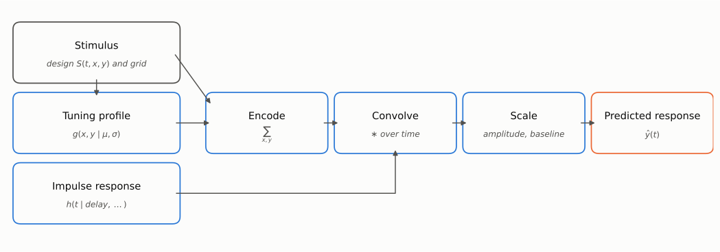
Figure 1. The canonical pRF model as a computational graph. The stimulus design and the parameterized submodels (blue) enter a chain of operations that ends in a predicted response.
Population tuning
The core set of submodels describe the tuning profile of neuron populations (e.g., all neurons located within a voxel in fMRI) towards experimental stimuli (e.g., a bar passing through the visual field). For example, for visual pRF models, the tuning profile is also called the receptive field that is the “region in visual space that stimulates the recording site” (p. 647)[1][2]. For connective field models, the tuning profile is the stimulation by neuron populations in a source area (e.g., V1)[3].
Tuning profiles are defined on the feature space of the experimental stimulus. For visual pRF models, the feature space is typically the 2D visual field (measured in degrees of visual angle). However, for other modalities, the feature space can be different: For example, numerosity (e.g., the number of objects seen by the subject)[4] or auditory stimuli are typically defined in 1D logarithmic feature spaces (measured in log integers or log frequency). Connective field models are always defined on the 2D geodesic distance matrix of the source region.
More advances tuning profiles also account for static nonlinearities, such as surround-suppression (difference of Gaussian)[5] or saturation (compressive spatial summation)[6] or both (divisive normalization)[7].
Figure 2. The same Gaussian tuning model on two feature spaces
(Gaussian2DPRFTuning on the left,
Gaussian1DPRFTuning on the right). Drag the slider to change the tuning width;
each panel shows the width on the scale of its own feature space. For the purpose of this visualization, both profiles
are normalized to their peak. prfmodel normally uses proper densities that are not peak-normalized (see
Important details).
Stimulus encoding
To predict a temporal neural response, population tuning profiles are often encoded by the design of the experimental stimulus. For example, for visual pRF models, the design describes the activity in the visual field over time (e.g, the location of a bar). The design is the component that drives the response of a neuron population in relation to the feature space of the stimulus. Computationally, the encoding differs between model families: For example, visual pRF models use the dot product to encode the pRF tuning profile with the stimulus design.
Connective field models do not explicitly use the stimulus design for encoding. Instead they encode the connective field tuning profile with the neural responses in the source region (i.e., the source region is the “stimulus”). However, the source region neural responses are usually elicited through an actual experimental stimulus that is then implicitly encoded in the connective field response.
Figure 3. Encoding a pRF tuning profile (orange contours) with a moving bar design
(encode_prf_response()). Drag the slider through the experiment: the response on the
right peaks whenever the bar overlaps the pRF.
Impulse response convolution
Depending on how the observed neural responses are measured (e.g., with fMRI), the stimulus-encoded neuron population responses must be modified to resemble the canonical shape that is inherent to the measurement. For example, BOLD response measurements in fMRI have a canonical shape following the hemodynamic response function (HRF). To bring the raw stimulus-encoded neural responses into the measurement space of the observed timecourses, they are usually convolved with an impulse response. Impulse models predict a response over a short time period that has the canonical shape of the measurement (e.g., the HRF is typically defined over a duration of 20-30 seconds). The convolved response then contains the stimulus-encoded neuron population response but also follows the canonical shape of the measurement. Note that the convolution is linear, an assumption that can be violated under rapid or brief stimulus presentations. Advanced models, such as delayed normalization[8] or compressive spatio-temporal models[9][10], address these problems.
Connective field models already exhibit the measurement shape in the neural responses of the source region so they usually do not need the convolution with the impulse response.
Figure 4. Convolving the encoded response with a derivative two-gamma impulse response
(DerivativeTwoGammaImpulse). Drag the slider to move the weight of the derivative of the
impulse response: the convolved response (orange) is a time-shifted and smoothed version of the encoded response
(blue).
Scaling
To bridge differences in baseline and scaling between predicted model responses and observed timecourses, model predictions are typically scaled and/or shifted. For some models, amplitude and baseline parameters that define the scaling and offset are treated as nuisance parameters. In other models (e.g., difference of Gaussian and divisive normalization models), amplitudes are treated as interpretable parameters and only baseline parameters as nuisances.
Figure 5. Scaling the (peak-normalized) convolved response with BaselineAmplitude.
The dotted line is the unscaled response.
Fitting
In prfmodel, a model that makes predictions can be compared to observed neural responses to optimize the model parameters and minimize the discrepancy between the two. The package provides several fitting methods that are best applied in sequence (this part has been inspired by the braincoder Python package).
The standard fitting workflow starts with a grid search over the core parameters of the model. For example, in the visual Gaussian pRF model, the core parameters are the center of the Gaussian (i.e., the mean) and the size of the receptive field (i.e., the standard deviation). By casting a wide grid, the search ensures that the core model parameters estimates fall in the region that provides predictions that are close to the observed data. The grid search is followed by least-squares estimation of baseline and amplitude parameters. Finally, some or all model parameters are finetuned with stochastic gradient descent (SGD) using the estimates from the previous stages as starting values. SGD is efficient at scale and benefits from the GPU-accelerated backends.
Because model fitting is fast, users can quickly iterate through the fitting stages and move from simple models to
incrementally more complex ones. The Getting started page walks through this workflow with
GridFitter, LeastSquaresFitter, and
SGDFitter.
Diagnostics
After models are fit to observed data and parameters are estimated, prfmodel helps the user to assess the quality of the fit and parameter estimates.
What prfmodel is not
prfmodel is not a package for preprocessing neuroimaging data since this is already extensively covered by other software and would massively blow up the scope of the package. For the same reasons, it is also not designed to be a package for visualizing neuroimaging data. We instead rely on nilearn for this task, but also suggest that MacOS and Linux users experiment with pycortex for visualization.